MODEL TRAINING

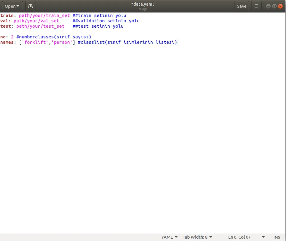
Model training varies depending on the algorithm being used. For YOLO, which is the most preferred due to its speed and performance, the training process proceeds as follows: After preparing the dataset, a YAML file (data.yaml) must be created, specifying the paths of the datasets, the number of classes, and class names.

Once the dataset is ready, we need to choose a model. The model selection should consider the hardware specifications and the speed requirements for real-time performance. Our choice will be based on the YOLOv5 model. You can visit https://docs.ultralytics.com/ to review all YOLO models.
To summarize YOLOv5's general features:

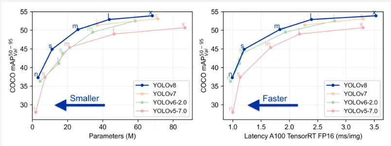
YOLOv5 builds on the performance of previous YOLO versions, with updated features for improved speed and accuracy. Its main advantage is its ease of use, which makes it accessible to a broad audience. Additionally, YOLOv5 supports transfer learning, allowing us to fine-tune pretrained models with new data. This improves performance and accelerates training. A comparison with other YOLO versions is shown in the graph below.

When using the YOLOv5 algorithm, we also need to choose among its internal models. YOLOv5 offers five primary model variants: n, s, m, l, and x. With version 6.x, additional versions (n6, s6, m6, l6, x6) were introduced, which are enhanced versions with more parameters and broader architecture. The key difference in this version is input image size:

• YOLOv5 uses 640 × 640
• YOLOv5.6 uses 1280 × 1280

This means that for more complex and larger images, YOLOv5.6 models will yield better performance. Below is a comparison of YOLOv5 model specifications.

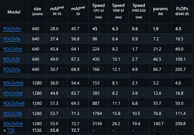
When analyzing YOLOv5 models, one of the most critical metrics is parameter count. This refers to the total weights and biases used during training and inference. The number of parameters determines a model’s learning capacity and complexity.

• More parameters make it easier to learn complex data relationships.
• However, this also increases the need for data and risks overfitting.
• More parameters require more computational power, longer training times, and larger model sizes.

Therefore, model selection should consider both the target application and hardware constraints. In our case, YOLOv5s meets the learning and real-time performance requirements, so we proceed with that.

Once the data is ready and the model selected, we need to clone the YOLOv5 repository. Ultralytics' website has detailed instructions, but the basic steps are as follows:

YOLOv5 Installation Steps

# Clone YOLOv5 Repository
git clone https://github.com/ultralytics/yolov5

# Enter YOLOv5 Directory
cd yolov5

# Install Requirements
pip install -r requirements.txt

After downloading the YOLOv5 repo, entering the folder, and installing dependencies, we can start training:

train.py --data ./data.yaml --epochs 300 --weights 'yolov5s.pt'  --cfg models/yolov5s.yaml --batch-size 128

Explanation of parameters:

• --data: Path to the custom data.yaml file which contains dataset info.
• --epochs: Number of training epochs (in our case, 300 full dataset passes).
• --weights: Path to pretrained weights to start training from. Leave empty for training from scratch.
• --cfg: Path to model config file. This must be edited to reflect the number of classes. It also defines layers, filters, learning rates, and more.
• --batch-size: Number of images processed per iteration. Larger values speed up training but increase memory usage.

Adjust these parameters according to your project and device, then begin training.

While or after training, go to the runs/train/exp folder inside the YOLOv5 directory to access training output graphs. An example is shown below:

• Box: Shows the accuracy of predicted bounding boxes. A value approaching 100 indicates that predicted boxes closely match ground truth.
• Objectness: Measures how well the model predicts object presence. Closer to 100 means more accurate detections in object areas.
• Classification: Indicates the accuracy of class predictions for detected objects. A higher score reflects strong classification ability.
• Precision: Proportion of correct positive predictions among all positive predictions made.
• Recall: Proportion of correct positive predictions among all actual positives.
• Val Box: Validation set bounding box prediction accuracy; allows comparison between training and validation performance.
• Val Objectness: Objectness prediction accuracy on the validation set.
• Val Classification: Classification accuracy on the validation set.
• mAP@0.5: Mean Average Precision at IoU 0.5; a key indicator of model performance.
• mAP@0.5:0.95: Mean Average Precision averaged over IoU thresholds from 0.5 to 0.95; more comprehensive metric.

After evaluating model performance via these graphs, we can proceed to real-time inference if needed:

detect.py --weights '' --source 0

Explanation of real-time inference parameters:

• --weights: Path to the trained model to be used for inference.
• --source: Input source for object detection. Some valid examples:
  • "0" → webcam
  • "img.jpg" → single image
  • "vid.mp4" → video
  • "path/" → folder
  • "list.txt" → list of images
  • "list.streams" → list of video streams
  • 'https://www.youtube.com/@cozummakina1538' → YouTube
  • 'rtsp://example.com/media.mp4' → RTSP, RTMP, HTTP stream

#yolov5 #yolov5spt #TransferLearning #datayaml #ParameterCount #DeepLearning #GPU #Ultralytics #weights #config #epochs #batchsize #loss #recall #mAP05 #mAP0595